RAG with ColPali: theory, implementation, and production tips
In this article I’ll walk you through the ColPali model, a multimodal embedding model released in 2024, and the pros and cons of choosing it for your Retrieval-Augmented Generation (RAG) pipeline.
Introduction
RAG is an essential component in any AI assistant that relies on static documents. However, many of those documents are visually rich , containing tables, images, formulas, charts, and so on, which makes multimodal search essential.
In real-world scenarios, the bottleneck in a RAG system rarely comes from the LLM; it comes from data ingestion and retrieval.
We will see how ColPali solves this problem in a unified way.
Motivation
To understand the motivation behind ColPali, we need to walk through the RAG pipeline. A RAG pipeline has two steps: offline and online.
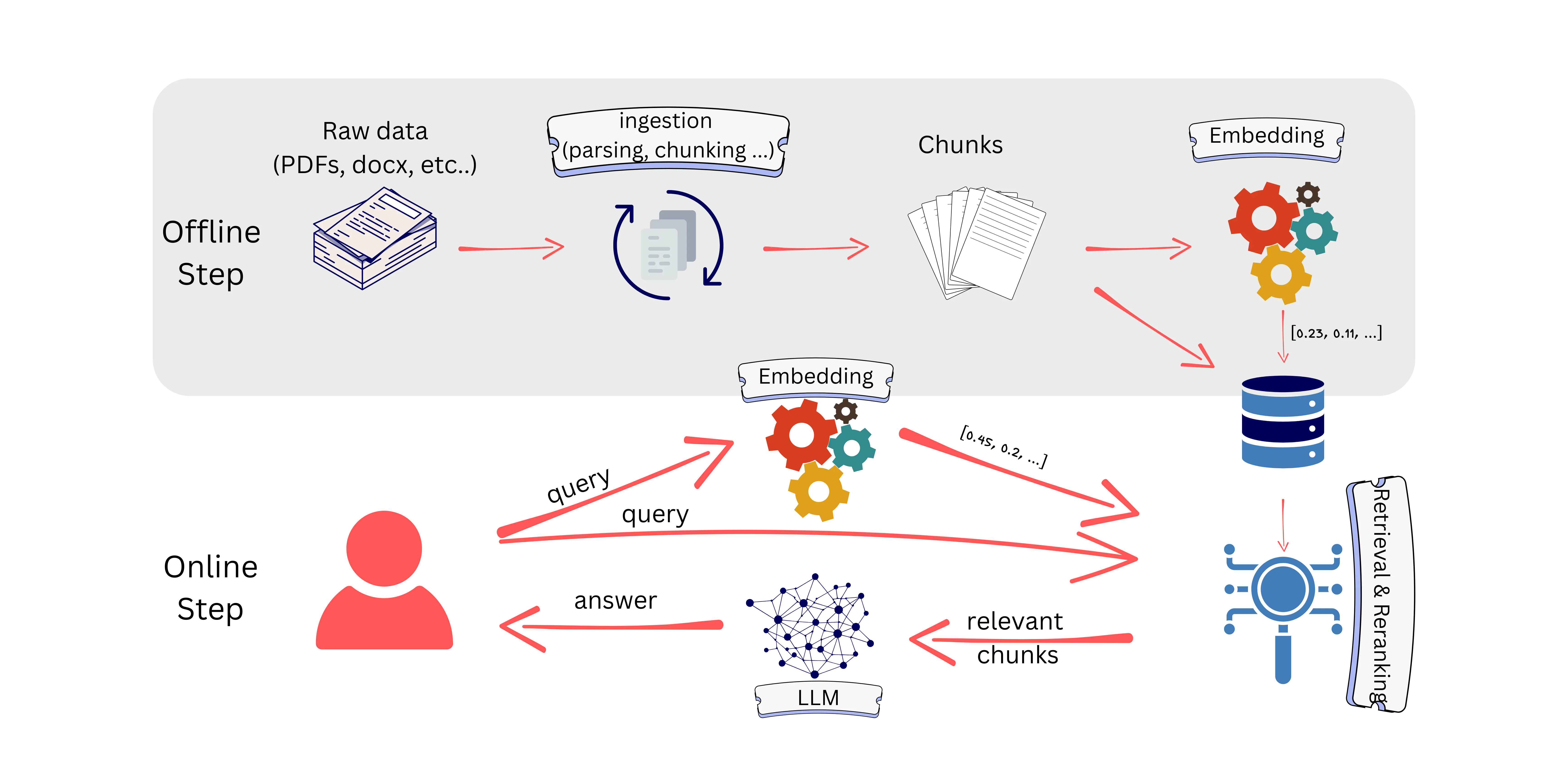
The offline step consists of data ingestion and embedding. Data ingestion transforms raw data (in our case, visually rich documents) into chunks. Those chunks are then converted into embeddings and stored in a database.
Once ready, the user asks a question; the goal is to retrieve the chunks most similar to the user’s query and send them to the LLM.
Because our documents are visually rich, they may include images, tables, formulas, scanned pages, charts, etc. These elements contain a lot of information, so we need to convert them into embeddings as well.
Some approaches convert those elements into text:
- Convert tables to Markdown.
- Convert formulas to LaTeX.
- Describe images with captions.
- Extract scanned text with OCR.
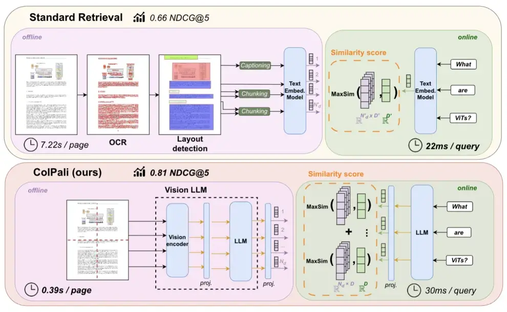
ColPali is a vision–language model trained for document retrieval. It directly converts a document page into embeddings, whether the page contains text, images, tables, or any combination of them.
By doing this, it removes the costly data-ingestion step and makes the offline part of a RAG pipeline much faster.
What is ColPali?
ColPali is a vision-language model trained for document retrieval. It directly converts a document page into embeddings, whether the page contains text, images, tables, or any combination of them.
By doing this, it removes the costly data-ingestion step and makes the offline part of a RAG pipeline much faster.
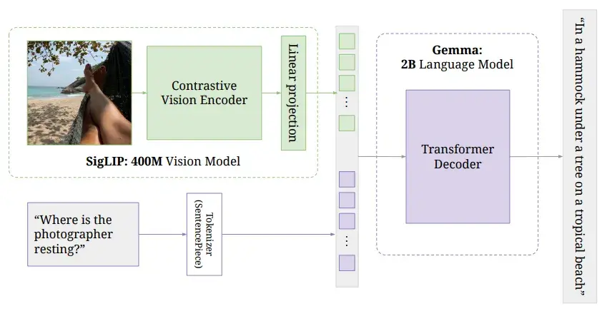
The name ColPali refers to two components: ColBERT and PaliGemma. PaliGemma is a vision–language model trained to generate text from a given image and accompanying text inputs as follows:
ColBERT refers to the output style used for late interaction (see next section).
ColPali fine-tunes PaliGemma for retrieval: it starts from the weights of a trained vision encoder and an LLM, and fine-tunes them to produce embedding vectors.
It may confuse people to see an LLM used for embeddings since it is decoder-only. By removing the classifier/head used for generation, a fine-tuned LLM can be used as an embedding model (without performing autoregressive generation).
By taking out the classifier head, a finetuned LLM for retrieval can be used as an embedding model
ColPali can take as input either a document page (an image) during the offline indexing stage or a user query (text) at retrieval time.
It is fine-tuned with a contrastive loss, so it outputs aligned text and image embeddings in the same latent space enabling cross-modal retrieval.
Late Interaction
We mentioned that ColPali combines ColBERT and PaliGemma. ColBERT is an embedding model similar to BERT, but it outputs multiple embedding vectors per input.
A standard BERT model takes a text input (a sentence, a paragraph, etc.) and generates a single embedding vector representing that input. A ColBERT model takes a text input and generates a vector per token, so if the input has 100 tokens, we get 100 vectors representing the input.
Late interaction is a middle step between embedding and reranking.
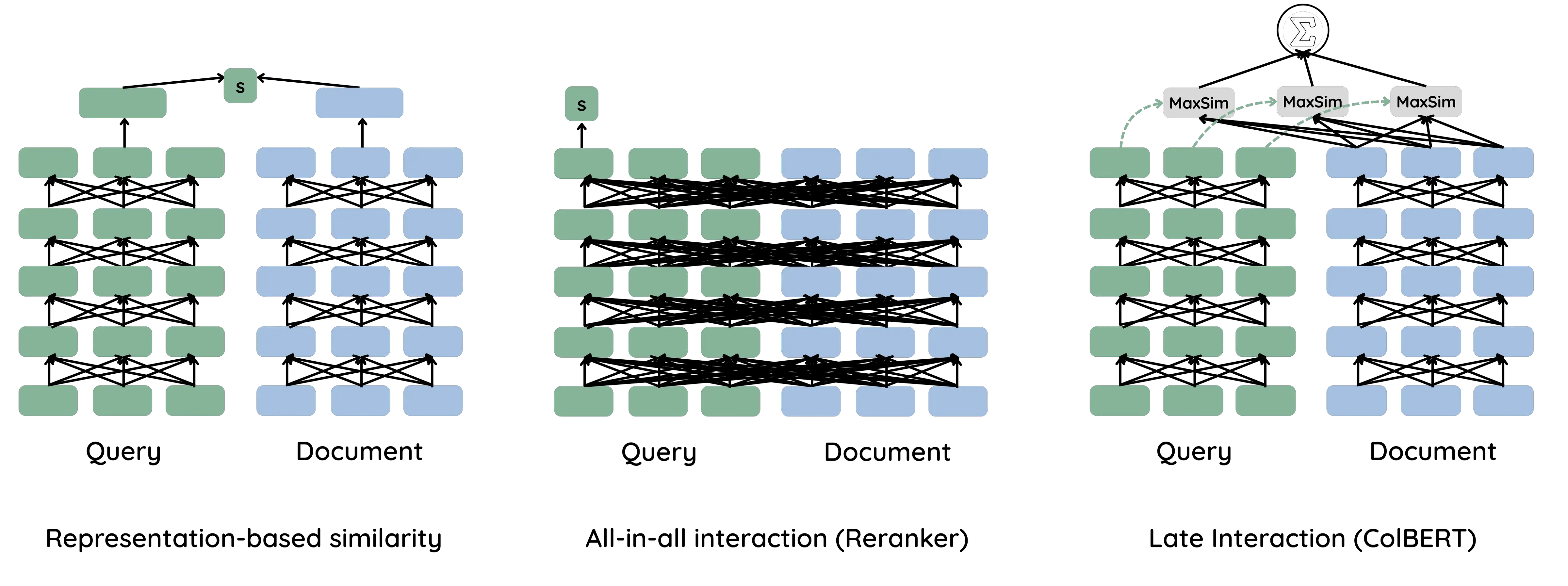
An embedding model like BERT compares a query and a document using their final embeddings without any direct interaction inside the network. A reranker, on the other hand, concatenates the query and the document so the network can see them together to assess similarity.
There is a trade-off between speed and precision. An embedding-based approach is fast because we compute document embeddings only once, but it can be less precise since the model never sees the <query, document> pair together. A reranker is more precise but slower, because we must recompute the similarity for each <query, document> pair.
Late interaction sits in the middle: it is fast, we compute the embeddings once for the document, but it is also precise because we have multiple representatives (multiple embedding vectors) for the query and the document.
In this setup, we compute the maximum similarity across token vectors to assess <query, document> similarity (more on this later).
This mechanism makes a lot of sense for ColPali. As mentioned before, ColPali consumes an entire document page as input. A page can contain different kinds of information that cannot be captured by a single vector. By generating multiple vectors, we increase the chance of matching the specific section of the page that is relevant to a user query.
Late interaction also solves the problem of choosing chunk size. Instead of opting for a single-vector representation per chunk, we generate multiple vectors, eliminating the effect of chunk size on retrieval precision.
Note that each embedding in ColBERT is typically small, about 128 dimensions, to limit computational cost.
ColPali Engine
ColPali Engine is the library used to fine-tune ColPali. Let’s see how it can be used in practice.
Suppose I want to generate embeddings for the ColPali paper pages. We start by converting each page into an image.
import pymupdf
from PIL import Image

def convert_pages_to_images(document_path):
    document = pymupdf.open(document_path)
    for page in document.pages():
        pix = page.get_pixmap()
        img = Image.frombytes("RGB", [pix.width, pix.height], pix.samples)
        yield img
    document.close()

# img.size = (612, 792)
Now we call the processor, which can handle image or text. We’ll use ColQwen2.5 with weights from Metric-AI.
from colpali_engine.models import ColQwen2_5_Processor

model_name = "Metric-AI/ColQwen2.5-3b-multilingual-v1.0"
processor = ColQwen2_5_Processor.from_pretrained(model_name, use_fast=True)

processed_img = processor.process_images([image])

# processed_img keys: {'pixels_values', 'image_grid_thw', 'input_ids', 'attention_mask'}
The processed_img object contains the attributes used by the vision encoder: pixel_values, image_grid_thw, and input_ids.
Let’s check the dimensions of each attribute:
| img size | image_grid_thw | pixels_values size | input_ids |
|---|---|---|---|
| (1, 612, 792, 3) | (1, 56, 44) | (1, 2464, 1176) | (1, 627) |
To understand how those values are calculated, check preprocessor_config.json:
{
  "do_convert_rgb": true,
  "do_normalize": true,
  "do_rescale": true,
  "do_resize": true,
  "image_mean": [
    0.48145466,
    0.4578275,
    0.40821073
  ],
  "image_processor_type": "Qwen2VLImageProcessor",
  "image_std": [
    0.26862954,
    0.26130258,
    0.27577711
  ],
  "max_pixels": 12845056,
  "merge_size": 2,
  "min_pixels": 3136,
  "patch_size": 14,
  "processor_class": "ColQwen2_5Processor",
  "resample": 3,
  "rescale_factor": 0.00392156862745098,
  "size": {
    "longest_edge": 12845056,
    "shortest_edge": 3136
  },
  "temporal_patch_size": 2
}
The most important parameters here are patch_size=14, merge_size=2, and temporal_patch_size=2.
Our image is decomposed into patches of size 14, that’s how we get image_grid_thw (a smart_resize adapts the image size so the grid dimensions are integers).
pixel_values holds the values for each patch. We have 56 * 44 = 2464 patches; each patch covers 14 * 14 * 3 = 588 pixels. However, the pixel_values array shows 1176 values per patch because temporal_patch_size is set to 2 (a parameter originally intended for videos), so the pixel values are duplicated: 14 * 14 * 3 * 2 = 1176.
By dropping the redundant temporal dimension, we can reconstruct the original image from those pixel values.
The last — and most important — parameter is input_ids. In the PaliGemma model we provide an image plus a text prompt describing the image. In ColPali we do the same: we use a fixed input prompt as follows:
"<|im_start|>user\n<|vision_start|><|image_pad|><|vision_end|>Describe the image.<|im_end|><|endoftext|>"There are special tokens added during fine-tuning:
{
  "</tool_call>": 151658,
  "<tool_call>": 151657,
  "<|box_end|>": 151649,
  "<|box_start|>": 151648,
  "<|endoftext|>": 151643,
  "<|file_sep|>": 151664,
  "<|fim_middle|>": 151660,
  "<|fim_pad|>": 151662,
  "<|fim_prefix|>": 151659,
  "<|fim_suffix|>": 151661,
  "<|im_end|>": 151645,
  "<|im_start|>": 151644,
  "<|image_pad|>": 151655,
  "<|object_ref_end|>": 151647,
  "<|object_ref_start|>": 151646,
  "<|quad_end|>": 151651,
  "<|quad_start|>": 151650,
  "<|repo_name|>": 151663,
  "<|video_pad|>": 151656,
  "<|vision_end|>": 151653,
  "<|vision_pad|>": 151654,
  "<|vision_start|>": 151652
}
Looking at the input_ids content, it contains the tokens for the input sentence, with the special token image_pad repeated 616 times.
processed_img['input_ids'].unique_consecutive()
# [151644, 872, 198, 151652, 151655, 151653, 74785, 279, 2168, 13, 151645, 151643]
(processed_img['input_ids'] == 151655).sum() # 616
The number of image_pad tokens corresponds to the vision tokens fed to the vision encoder.
We started with 2464 patches, but because merge_size=2 is applied in both x and y directions, the vision token count is reduced by a factor of 4: 2464 / 4 = 616 vision tokens, plus 11 special tokens = 627 total tokens.
Once the input image is prepared, we feed it to ColPali:
import torch
from colpali_engine.models import ColQwen2_5

model_name = "Metric-AI/ColQwen2.5-3b-multilingual-v1.0"
model = ColQwen2_5.from_pretrained(
    model_name,
    torch_dtype=torch.bfloat16,
    device_map="cuda:0",
).eval()

embeddings = model(**processed_img)

# embeddings.shape = (627, 128)
The input image is converted into 627 embedding vectors, each of size 128.
Now let’s see how we can process and generate embeddings for an input text:
import torch
from colpali_engine.models import ColQwen2_5_Processor, ColQwen2_5

model_name = "Metric-AI/ColQwen2.5-3b-multilingual-v1.0"

processor = ColQwen2_5_Processor.from_pretrained(model_name, use_fast=True)
model = ColQwen2_5.from_pretrained(
    model_name,
    torch_dtype=torch.bfloat16,
    device_map="cuda:0",
).eval()


query = "What is ColPali?"

processed_query = processor.process_texts([query]).to(model.device)
# {'input_ids': tensor([[3838,  374, 4254,   47, 7956,   30]], device='cuda:0')}

query_embeddings = model(**processed_query)
# query_embeddings.shape = (6, 128)
MaxSim
After generating embeddings for all document pages, and for the query we need to find the pages most similar to the query. To do that we use the maximum similarity metric.
MaxSim works like this: compare each query embedding (each vector of dimension 128) to all embeddings of a page (for example, the 627 vectors of dimension 128) using cosine similarity. For one query token you get 627 cosine-similarity values; you take the maximum of those 627 values.
Repeat that for every query token (e.g., if the query has 6 tokens, you’ll get 6 maxima), and then aggregate those maxima into a single score for the query–page pair by summing them.
This can be implemented efficiently as a matrix operation.
Denote E_Q and E_P the embedding matrices of the query and the page, with E_Q.shape=(n_text_tokens, d) and E_P=(n_visual_tokens, d) where d is the embedding dimension (128 in our case).
If embeddings are L2-normalized, the maximum similarity is simply
max_sim = (E_Q@E_P.T).max(axis=1).sum(axis=0)Important points about maximum similarity:
- Query-length dependence.
max_simis not bounded: it takes the best match for each query token and then aggregates those values. That means the final score grows with the number of query tokens (in practice, per-token maxima tend to be non-negative) so longer queries often score higher just because they contain more tokens. This is not a problem by itself because we generally don’t compare scores across queries, but I prefer averaging the per-token maxima rather than summing, so the score is bounded between [-1, 1]. - Asymmetry.
max_sim(q, d)is different thanmax_sim(d, q).
Don’t confuse the query-length dependence with image-length dependence. Max Sim handles images of different sizes well, so you don’t need to resize all your images to the same size.
Approximate Search
One problem with having multiple embedding vectors per page is that indexes like HNSW or IVFFLAT don’t support this directly. In practice we almost always use approximate search instead of exact search, so we need a way to make retrieval fast with ColPali.
Some vector databases have added native support for late interaction and MaxSim (for example rank_vectors type in Elasticsearch), but here I’ll show how to implement it in plain SQL using PostgreSQL + pgvector.
The code below is taken from pgvector's official examples for ColBERT models (the same code works for ColPali).
If you don't know what pgvector is or how to use it, check the ultimate guide to using pgvector.
First, create two tables: one for page metadata (document id, content, etc.) and one for embedding vectors. We store the embeddings of a single page in multiple rows, so it’s a one-to-many relationship.

Next, define the max_sim function:
CREATE OR REPLACE FUNCTION max_sim(document vector[], query vector[]) RETURNS double precision AS $$
    WITH queries AS (
        SELECT row_number() OVER () AS query_number, *
        FROM (SELECT unnest(query) AS query)
    ),
    documents AS (
        SELECT unnest(document) AS document
    ),
    similarities AS (
        SELECT query_number, 1 - (document <=> query) AS similarity
        FROM queries CROSS JOIN documents
    ),
    max_similarities AS (
        SELECT MAX(similarity) AS max_similarity
        FROM similarities GROUP BY query_number
    )
    SELECT SUM(max_similarity) FROM max_similarities
$$ LANGUAGE SQL
The max_sim function takes two inputs: a document page and a query, both represented as arrays of vectors. It builds four CTEs:
queriesa list of separated query vectors (unnest) with their enumeration (query_number).documents: a list of separated page vectors.similarities: the cosine similarity (1 — cosine distance) and the query number between each (cross join) query vector and page vector.max_similarities: group the similarities byquery_numberand keep the maximum for each query token.
Finally the function returns the SUM (or SUM>) of those per-token maxima.
So far this is just the max_sim computation; we haven’t done any approximation yet. The trick is to first select a subset of candidate pages using a fast approximate search, then run max_sim only on those candidates. That’s done here:
approximate_stage = ' UNION ALL '.join(['(SELECT document_id
                                          FROM document_embeddings
                                          ORDER BY embedding <=> %s
                                          LIMIT 5)'
                                 for _ in query_embeddings])
For each query embedding we select the top-5 pages (by document_id) based on cosine similarity with that single query embedding. If a query has 10 tokens, we run this for each token and return up to 5 page IDs per token.
This stage uses the index to do approximate nearest-neighbor search (cosine between two vectors), not MaxSim.
Note that returned page IDs are not necessarily distinct — different query tokens can vote for the same page.
We use UNION ALL so this runs as a single SQL query.
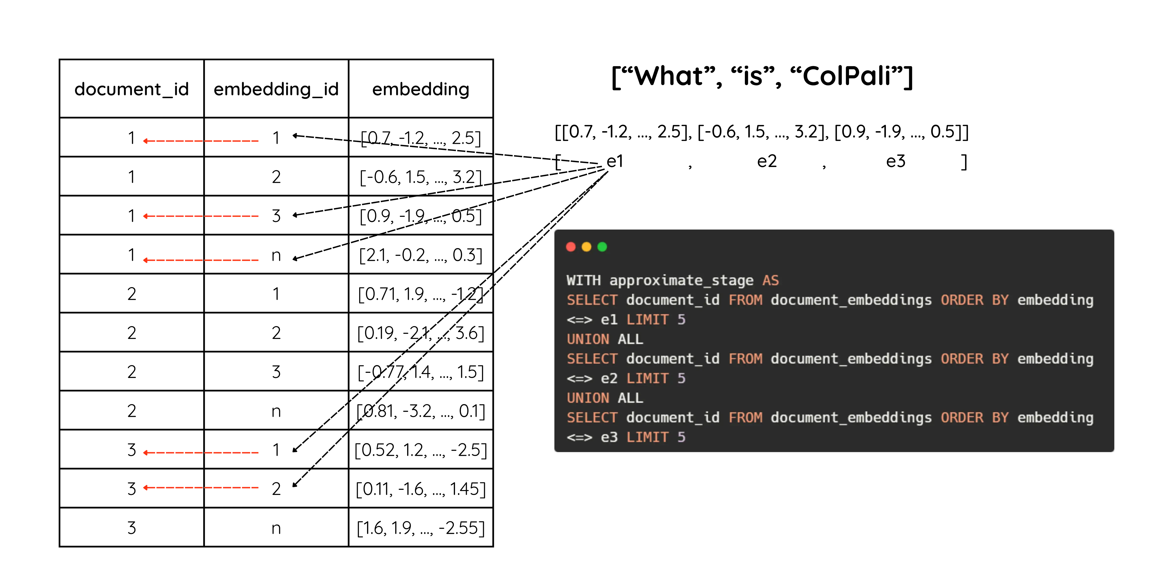
Finally we aggregate the returned page embeddings and compute max_sim:
WITH approximate_stage AS (
    {approximate_stage}
),
embeddings AS (
    SELECT document_id, array_agg(embedding) AS embeddings FROM document_embeddings
    WHERE document_id IN (SELECT DISTINCT document_id FROM approximate_stage)
    GROUP BY document_id
)
SELECT content, max_sim(embeddings, %s) AS max_sim FROM documents
INNER JOIN embeddings ON embeddings.document_id = documents.id
ORDER BY max_sim DESC LIMIT 10
Here we define two CTEs:
-
approximate_stage: the list ofdocument_id(page numbers) found in the approximate step. -
embeddingsdocument_idand the concatenated embedding vectors (array_agg(embedding)) for each page found inapproximate_stage.
With embeddings available, we call max_sim on the grouped embeddings and the query (the query is passed as %s). The example performs an INNER JOIN to fetch the document content from the documents table (the example was written for ColBERT).
In short: first do an approximate search to produce a small set of candidate pages, then compute
max_simon those candidates and return the most similar page(s).
Token Pooling
If you’ve followed this far, you might have felt we’re generating a lot of vectors per page — 627 vectors per page in our earlier example. So instead of storing and retrieving a single vector per page, we have 627. For a 200-page document, that’s 200 × 627 = 125,400 vectors!
This is one downside of ColPali. Luckily there’s a simple way to reduce the vector count: pooling. The idea is to cluster nearby vectors and take their average. Since our patches are small (14×14), many vectors cover blank or meaningless areas (white margins, etc.), so pooling helps a lot.
There are several pooling strategies; here we focus on hierarchical clustering.
import torch
from colpali_engine.models import ColQwen2_5, ColQwen2_5_Processor
from colpali_engine.compression.token_pooling import HierarchicalTokenPooler

# create processor, model and pooler objects
model_name = "Metric-AI/ColQwen2.5-3b-multilingual-v1.0"
processor = ColQwen2_5_Processor.from_pretrained(model_name, use_fast=True)
model = ColQwen2_5.from_pretrained(
    model_name,
    torch_dtype=torch.bfloat16,
    device_map="cuda:0",
).eval()
pooler = HierarchicalTokenPooler()

# process the image
processed_img = processor.process_images([img]).to("cuda:0")

# generate embeddings
embeddings = model(**processed_img)
# embeddings.shape = (1, 627, 128)

# cluster embeddings
pooled_embeddings = pooler.pool_embeddings(embeddings, pool_factor=2, return_dict=False)
# pooled_embeddings.shape = (1, 313, 128)
As we can see, using a pool_factor of 2 halves the number of embedding vectors. That produces 313 clusters, and we aggregate each cluster into a single vector. You can access the cluster information by setting return_dict=True.
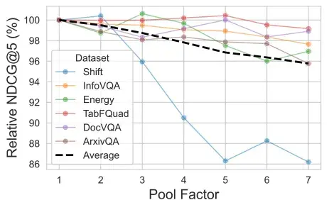
As stated in the paper, vector reduction incurs only a small performance degradation.
“With a pool factor of 3, the total number of vectors is reduced by 66.7% while 97.8% of the original performance is maintained.”
Practical Aspects
There are several practical aspects to consider when deciding to use ColPali:
- Retrieval speed
- Hybrid search
- LLM consumption
- Model serving
ColPali is fast when it comes to indexing because it completely removes the document-ingestion step. However, since each page produces multiple vectors, retrieval speed becomes a real concern.
ColPali can increase the number of vectors by roughly 100× if you currently handle 10 million vectors, you’ll need to manage about 1 billion. Many vector databases don’t scale efficiently to that level, so it’s important to evaluate your infrastructure.
In addition, considering hybrid search (keyword + embedding). You can extract text from document pages to perform keyword search, but how do you re-rank the results? Cross-encoder models are generally not multimodal, so reranking across text and image isn’t straightforward.
Another issue involves LLM consumption. The retrieved chunks from ColPali are images: how will your LLM consume them? Should they be passed directly as images, or should you apply a data ingestion step before feeding them to the LLM? Also keep in mind that image tokens are usually more expensive than text tokens.
Finally, for production use, you’ll need a serving library like vLLM to handle concurrent requests. Unfortunately, at the time of writing, vLLM doesn’t yet support late-interaction models such as ColPali. However, I managed to modify the vLLM code to serve the model I’m using, and it worked efficiently. Check the GitHub issue here.
To conclude, ColPali is an excellent choice for building RAG systems on visually rich documents. It removes the need for data ingestion by directly embedding each page into a set of vectors.
However, it also adds complexity to the retrieval stage and can increase LLM consumption, since the model may need to process images instead of plain text.
References
- Faysse, M., et al. (2024). ColPali: Efficient Document Retrieval with Vision Language Models
- Khattab, O., & Zaharia, M. (2020). ColBERT: Efficient and Effective Passage Search via Contextualized Late Interaction over BERT
- Beyer, L., et al. (2024). PaliGemma: A versatile 3B VLM for transfer
- ColPali Engine
- ColQwen2.5-3b-multilingual-v1.0
- PGVector Python Examples