The Ultimate Guide to using PGVector
In this comprehensive guide, I’ll show you how to use pgvector on a database table containing millions of rows and ensure you’re doing so efficiently. I’ve made some unintuitive mistakes along the way so you don’t have to. Here’s what we’ll cover:
Introduction
Let’s start by looking at the setup. I built a Python web app using Dash library to collect, visualize, and filter millions of news articles. (See screenshot of the app below.)

In the interface, you can filter articles by date, topic, source, and text. Under the hood, we store everything in a PostgreSQL database.
For keyword searches, we use PostgreSQL’s tsvector. For semantic search, we generate embeddings with a JINA model. pgvector is a PostgreSQL extension that makes it easy to store those embedding vectors and query for similar items. Next, we’ll see pgvector in action.
PGVector Setup
We use Docker and Docker Compose for this project. Here’s how we configure our Postgres service:
db:
  image: pgvector/pgvector:pg17 # we are using Postgres 17
  container_name: postgres_container
  environment:
    POSTGRES_USER: ${POSTGRES_USER}
    POSTGRES_PASSWORD: ${POSTGRES_PASSWORD}
    POSTGRES_DB: ${POSTGRES_DB}
  volumes:
    - postgres_data:/var/lib/postgresql/data
    - ./schema.sql:/docker-entrypoint-initdb.d/schema.sql
When the container starts, the environment variables set up the database user, password, and name. The ./schema.sql file runs once at startup and creates the pgvector extension:
CREATE EXTENSION IF NOT EXISTS vector;At this point, we have a fresh database with pgvectorenabled. Next, we’ll set up our table.
Table Creation
We’re using SQLAlchemy in this project. Below is the minimal code to create a table with a vector column:
from sqlalchemy import MetaData, Table, Column, BigInteger
from pgvector.sqlalchemy import Vector, HALFVEC

def create_table(engine, table_name):
  metadata = MetaData()
  table_ref = Table(
                table_name,
                metadata,
                Column(
                    DBCOLUMNS.rowid.value,
                    BigInteger,
                    primary_key=True,
                    autoincrement=True,
                ),
                .
                .
                .
                Column(
                    DBCOLUMNS.embedding.value, # the column name
                    HALFVEC(VECTOR_DIM), # the column type
                    nullable=True,
                ))
    metadata.create_all(engine)
    return table_ref
First, install the pgvector package by running pip install pgvector.
Once that’s done, import the types you need:
from pgvector.sqlalchemy import Vector, HALFVEC
In our create_table function, we use HALFVEC, which stores vectors in half precision.
According to the pgvector documentation, the supported column types are:
vector: up to 2,000 dimensionshalfvec: up to 4,000 dimensionsbit: up to 64,000 dimensionssparsevec: up to 1,000 non-zero elements
These limits refer to the size of the embedding vector your model produces. In our case, we use a 1,024-dimensional vector. If you need variable-length vectors, use HALFVEC without specifying a dimension (instead of something like HALFVEC(1024)). Note that variable-length vectors can’t be indexed (we’ll cover indexing later).
When we collect data, we compute the embedding for each news article’s body using the JINA model and store it in the embedding column. Once that column is filled, you can calculate similarity distances between an embedded query and the stored embeddings.
Querying The Column
Let’s say you want to find news articles about “Israel crimes in Gaza” using the web app. First, you turn that search phrase into an embedding vector. Then you measure how close that query vector is to each article’s embedding.
pgvector supports several distance measures — inner_product, cosine_distance, euclidean_distance, and so on. Cosine distance is defined as 1 — cosine similarity. With these metrics, a smaller distance means the vectors are more similar; a larger distance means they’re less similar. This convention matters when we set up indexes (we’ll cover that soon).
In SQL, pgvector gives us special operators for these distances:
<#>for negative inner product<=>for cosine distance<->for Euclidean distance
Because JINA embeddings are already normalized, using the negative inner product is equivalent to using cosine distance. Here’s how you’d write a query to get the similarity score between your query’s embedding and every article’s embedding column:
SELECT rowid, (embedding <#> :query_vector) AS distance
FROM articles
WHERE embedding IS NOT NULL;
If you only want articles whose similarity score is below a certain threshold (remember, smaller is more similar), you can add a WHERE clause:
SELECT rowid, (embedding <#> :query_vector) AS distance
FROM articles
WHERE embedding IS NOT NULL
      AND (embedding <#> :query_vector) < 0;
Running this on a table with millions of rows means PostgreSQL has to scan every row and compute the distance for each one. On a large dataset, that can take few minutes. Clearly, we need a faster way and that’s where indexes come in.
Indexes
When you want to speed up a database operation, you usually reach for indexes, but it is a bit different for embedding columns.
In a vector database, you don’t get a speed up by just creating an index on the column. If you want to perform an exact nearest neighbor search to find all similar vectors, the index won’t help, but if you’re looking for an approximate search, an index can make a big difference.
There are multiple types of vector database indexes, but we will focus only here on Hierarchical Navigable Small Worlds (HNSW).
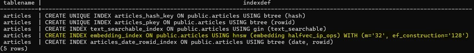
Here’s how to create an HNSW index on our embedding column:
CREATE INDEX articles_embedding_index ON articles
USING hnsw (embedding halfvec_ip_ops)
WHERE embedding IS NOT NULL;
In our setup, we’re using half-precision vectors (halfvec) and the negative inner product (ip) because our JINA embeddings are already normalized.
Make sure the index you create uses the exact same distance metric you plan to use when querying. If they don’t match, PostgreSQL won’t use the index.
Let’s see what happens when we run a query and check the execution plan. First, we store one of our existing embeddings in a variable:
-- Store the first embedding in a psql variable
SELECT embedding::text as query_vector
FROM articles
WHERE embedding IS NOT NULL
LIMIT 1 \gset
Then we run a similarity query against the table:
EXPLAIN (ANALYZE, BUFFERS, FORMAT TEXT)
SELECT
  rowid,
  (embedding <#> :'query_vector'::halfvec) AS distance
FROM articles
WHERE embedding IS NOT NULL
  AND (embedding <#> :'query_vector'::halfvec) < 0;
Here’s the query plan we got:
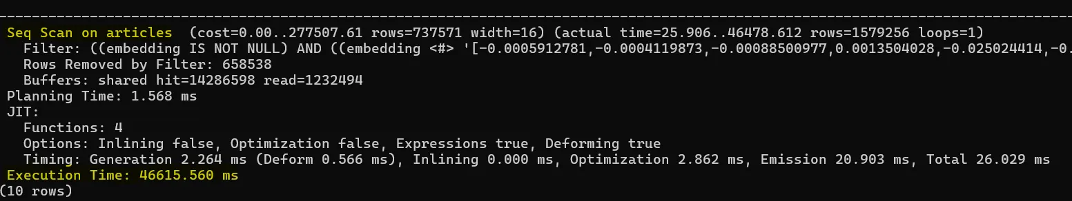
You’ll notice the planner did a sequential scan over 2.2 million rows and the query took 46 seconds. PostgreSQL ignored the HNSW index.
Approximate NN
To make PostgreSQL use the HNSW index, you need to run an approximate nearest neighbor search. In practice, that means two things in your SQL query:
- Include an
ORDER BY … LIMIT Kclause. - Sort in ascending order
ASC(the default order).
When the planner sees ORDER BY … LIMIT with the right ascending order, it knows to use the index. We use the negative inner product operator (<#>) so that smaller values—i.e., more similar vectors—come first. If you don’t use ORDER BY … LIMIT in ascending order, the index won’t be used.
If you don’t use
ORDER BY...LIMIT Kin your query in anASCorder, the index won’t be used.
The LIMIT K part tells PostgreSQL to return the top K nearest neighbors. Here’s the updated query:
EXPLAIN (ANALYZE, BUFFERS, FORMAT TEXT)
SELECT
  rowid,
  (embedding <#> :'query_vector'::halfvec) AS distance
FROM articles
WHERE embedding IS NOT NULL
  AND (embedding <#> :'query_vector'::halfvec) < 0
ORDER BY distance
LIMIT 100;
Below is the query plan when running this against our 2.2 million-row table:
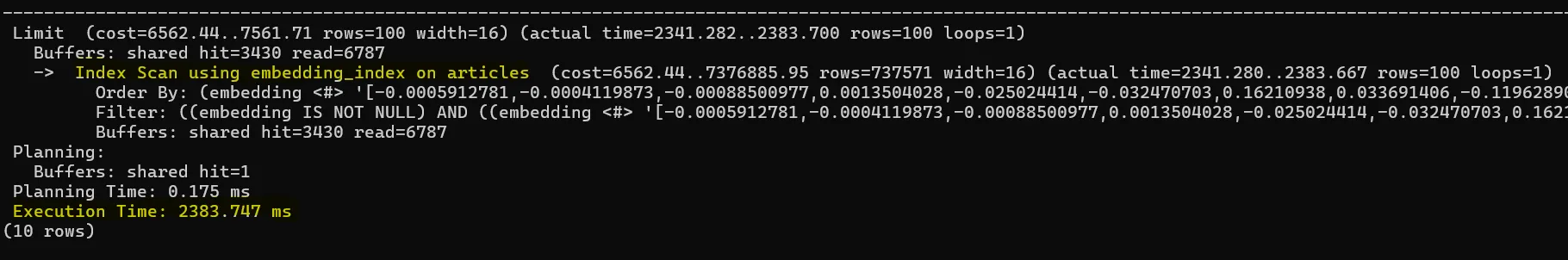
You can see the HNSW index is used, and the query finishes in about 2 seconds — much faster than a full scan. The number of rows you get back will be at most 100 (since we used LIMIT 100) and also depends on any WHERE clause (here, distance < 0).
Beyond those conditions, PostgreSQL also considers a parameter called ef_search that will limit the number of returned values as well.
HNSW Index
HNSW is a graph-based algorithm for approximate nearest neighbor (ANN) search. When you set up an HNSW index, you can adjust three key parameters:
- m: the maximum number of connections each node can have.
- ef_construction: how many candidates the algorithm considers when inserting a new point into the graph.
- ef_search: how many candidates the search explores when you run a query.
| Parameter | Build Time | Recall |
|---|---|---|
| m | ↑ (more neighbor comparisons) | ↑ (denser graph → higher recall) |
| ef construction | ↑ (larger candidate pool during insert) | ↑ (better link selection → higher recall) |
| ef search | — (no effect) | ↑ (more candidates → higher recall) |
If you want to dive into the details of how HNSW works, check out the original paper or a blog post that breaks down the algorithm step by step.
HNSW does not require a training phase like IVFFLAT. This means that we can create the index before having any data in the table, unlike IVVFLAT.
A good rule of thumb for a table with millions of rows is to set:
- m between 32 and 64
- ef_construction between 128 and 256
The ef_search parameter controls how many candidates the search will look at. In practice, you can’t ask for more nearest neighbors (your K in a KNN query) than the ef_search value.
For example, if ef_search is 200, you can request up to 200 nearest neighbors. The default ef_search is 40, but you can raise it up to a max of 1000 if you’re willing to trade a bit of extra query time for better recall:
SET hnsw.ef_search = 1000;Limitations
There are times when PostgreSQL can’t use the HNSW index, which means you lose the benefit of an approximate search. A common case is when you filter by attributes like date or source before doing the vector search.
For example, say you want to find articles about “Israel crimes in Gaza” but only those published before October 7. You might write:
EXPLAIN (ANALYZE, BUFFERS, FORMAT TEXT)
WITH filtered AS MATERIALIZED (
  SELECT
    rowid,
    embedding
  FROM articles
  WHERE
    embedding IS NOT NULL
    AND date < '2023-07-10'
)
SELECT
  rowid,
  (embedding <#> :'query_vector'::halfvec) AS distance
FROM filtered
WHERE
  (embedding <#> :'query_vector'::halfvec) < 0
ORDER BY distance
LIMIT 100;
In this query, PostgreSQL applies the date filter first, then calculates the vector distance on the remaining rows. Because the HNSW index was built over the entire table, it can’t be used here. Instead, PostgreSQL does a full scan of all rows where date < '2023-10-07', which is slow—especially on millions of rows.
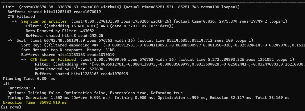
Logically, the planner skips the index because the index graph is built on all data, not just a subset. If you want the index to work, you need to let it run on the full dataset first and then apply filters.
One might try flipping the order — run the approximate search, then filter:
EXPLAIN (ANALYZE, BUFFERS, FORMAT TEXT)
SELECT
  rowid,
  (embedding <#> :'query_vector'::halfvec) AS distance
FROM articles
WHERE embedding IS NOT NULL
  AND date < '2023-07-10'
  AND (embedding <#> :'query_vector'::halfvec) < 0
ORDER BY distance
LIMIT 100;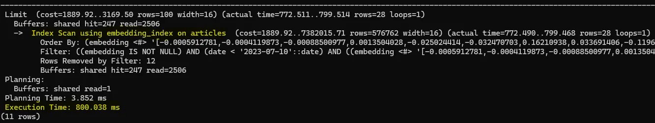
This lets the HNSW index find the 100 nearest neighbors before filtering by date. But now you risk losing recall: if most of those 100 aren’t from before October 7, you end up with very few (or zero) results.
To compensate, you’d have to increase the ef_search parameter so more candidates come back from the index—then hope enough fall within your date range.
In pgvector 0.8.0, we can increase the number of returned elements beyond ef_search using iterative scan
hnsw.iterative_scan.
Index lookups also break down when you use joins. For example, you might try to compare one embedding against all others with a CROSS JOIN. Unfortunately, in that scenario PostgreSQL can’t use the HNSW index, so it ends up doing a full-table scan instead.
EXPLAIN (ANALYZE, BUFFERS, FORMAT TEXT)
WITH first_vec AS (
  SELECT embedding AS query
  FROM articles
  WHERE embedding IS NOT NULL
  LIMIT 1
)
SELECT
  articles.rowid,
  articles.embedding <#> first_vec.query AS distance
FROM
  articles
  CROSS JOIN first_vec
WHERE
  articles.embedding IS NOT NULL
  AND (articles.embedding <#> first_vec.query) < 0
ORDER BY distance
LIMIT 100;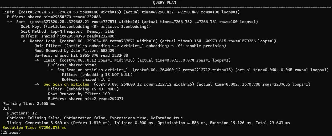
pgvector is a great way to add similarity search to your existing PostgreSQL database. Just be sure your index is used correctly so you get fast, reliable results.